In-class Exercise 2

Dr. Kam Tin Seong

26 Aug 2024

Getting started

• The task
• The code

For the purpose of this in-class exercise, tidyverseand sf packages will be used. Write a code chunk to check if these two packages have been installed in R. If yes, load them in R environment.

pacman::p_load(tidyverse, sf)

Working with Master Plan Planning Sub-zone Data

• The task
• The code

1. Create a sub-folder called data in In-class_Ex02 folder.
2. If necessary visit data.gov.sg and download Master Plan 2014 Subzone Boundary (Web) from the portal. You are required to download both the ESRI shapefile and kml file.
3. Write a code chunk to import Master Plan 2014 Subzone Boundary (Web) in shapefile and kml save them in sf simple features data frame.

This code chunk imports shapefile.

mpsz14_shp <- st_read(dsn = "data/",
                layer = "MP14_SUBZONE_WEB_PL")

Reading layer `MP14_SUBZONE_WEB_PL' from data source 
  `C:\tskam\IS415-GAA\In-class_Ex\In-class_Ex02\data' using driver `ESRI Shapefile'
Simple feature collection with 323 features and 15 fields
Geometry type: MULTIPOLYGON
Dimension:     XY
Bounding box:  xmin: 2667.538 ymin: 15748.72 xmax: 56396.44 ymax: 50256.33
Projected CRS: SVY21

This code chunk imports kml file.

mpsz14_kml <- st_read("data/MasterPlan2014SubzoneBoundaryWebKML.kml")

Working with Master Plan Planning Sub-zone Data

• The task
• The code

1. Write a code chunk to export mpsz14_shp sf data.frame into kml file save the output in data sub-folder. Name the output file MP14_SUBZONE_WEB_PL.

st_write(mpsz14_shp, 
         "data/MP14_SUBZONE_WEB_PL.kml",
         delete_dsn = TRUE)

Working with Pre-school Location Data

• The task
• The code

1. If necessary visit data.gov.sg and download Pre-Schools Location from the portal. You are required to download both the kml and geojson files.
2. Write a code chunk to import Pre-Schools Location in kml geojson save them in sf simple features data frame.

This code chunk imports kml file.

preschool_kml <- st_read("data/PreSchoolsLocation.kml")

This code chunk imports geojson file.

preschool_geojson <- st_read("data/PreSchoolsLocation.geojson") 

Working with Master Plan 2019 Subzone Boundary Data

• The task
• To import shapefile
• To import kml

1. Visit data.gov.sg and download Master Plan 2019 Subzone Boundary (No Sea) from the portal. You are required to download both the kml file.
2. Move MPSZ-2019 shapefile provided for In-class Exercise 1 folder on elearn to data sub-folder of In-class_Ex02.
3. Write a code chunk to import Master Plan 2019 Subzone Boundary (No SEA) kml and MPSZ-2019 into sf simple feature data.frame.

mpsz19_shp <- st_read(dsn = "data/",
                layer = "MPSZ-2019")

Reading layer `MPSZ-2019' from data source 
  `C:\tskam\IS415-GAA\In-class_Ex\In-class_Ex02\data' using driver `ESRI Shapefile'
Simple feature collection with 332 features and 6 fields
Geometry type: MULTIPOLYGON
Dimension:     XY
Bounding box:  xmin: 103.6057 ymin: 1.158699 xmax: 104.0885 ymax: 1.470775
Geodetic CRS:  WGS 84

mpsz19_kml <- st_read("data/MasterPlan2019SubzoneBoundaryNoSeaKML.kml")

Reading layer `URA_MP19_SUBZONE_NO_SEA_PL' from data source 
  `C:\tskam\IS415-GAA\In-class_Ex\In-class_Ex02\data\MasterPlan2019SubzoneBoundaryNoSeaKML.kml' 
  using driver `KML'
Simple feature collection with 332 features and 2 fields
Geometry type: MULTIPOLYGON
Dimension:     XY, XYZ
Bounding box:  xmin: 103.6057 ymin: 1.158699 xmax: 104.0885 ymax: 1.470775
z_range:       zmin: 0 zmax: 0
Geodetic CRS:  WGS 84

Handling Coordinate Systems

Checking coordinate system

• The task
• The code

Write a code chunk to check the project of the imported sf objects.

st_crs(mpsz19_shp)

Coordinate Reference System:
  User input: WGS 84 
  wkt:
GEOGCRS["WGS 84",
    DATUM["World Geodetic System 1984",
        ELLIPSOID["WGS 84",6378137,298.257223563,
            LENGTHUNIT["metre",1]]],
    PRIMEM["Greenwich",0,
        ANGLEUNIT["degree",0.0174532925199433]],
    CS[ellipsoidal,2],
        AXIS["latitude",north,
            ORDER[1],
            ANGLEUNIT["degree",0.0174532925199433]],
        AXIS["longitude",east,
            ORDER[2],
            ANGLEUNIT["degree",0.0174532925199433]],
    ID["EPSG",4326]]

Handling Coordinate Systems

Transforming coordinate system

• The task
• To import MPSZ-2019
• To import PreSchoolsLocation.kml

Re-write the code chunk to import the Master Plan Sub-zone 2019 and Pre-schools Location with proper transformation

mpsz19_shp <- st_read(dsn = "data/",
                layer = "MPSZ-2019") %>%
  st_transform(crs = 3414)

Reading layer `MPSZ-2019' from data source 
  `C:\tskam\IS415-GAA\In-class_Ex\In-class_Ex02\data' using driver `ESRI Shapefile'
Simple feature collection with 332 features and 6 fields
Geometry type: MULTIPOLYGON
Dimension:     XY
Bounding box:  xmin: 103.6057 ymin: 1.158699 xmax: 104.0885 ymax: 1.470775
Geodetic CRS:  WGS 84

preschool <- st_read("data/PreSchoolsLocation.kml") %>%
  st_transform(crs = 3414)

Reading layer `PRESCHOOLS_LOCATION' from data source 
  `C:\tskam\IS415-GAA\In-class_Ex\In-class_Ex02\data\PreSchoolsLocation.kml' 
  using driver `KML'
Simple feature collection with 2290 features and 2 fields
Geometry type: POINT
Dimension:     XYZ
Bounding box:  xmin: 103.6878 ymin: 1.247759 xmax: 103.9897 ymax: 1.462134
z_range:       zmin: 0 zmax: 0
Geodetic CRS:  WGS 84

Geospatial Data Wrangling

Point-in-Polygon count

• The task
• The code

Write a code chunk to count the number of pre-schools in each planning sub-zone.

mpsz19_shp <- mpsz19_shp %>%
  mutate(`PreSch Count` = lengths(
    st_intersects(mpsz19_shp, preschool)))

Geospatial Data Wrangling

Computing density

• The task
• The code

Write a single line code to perform the following tasks:

1. Derive the area of each planning sub-zone.

2. Drop the unit of measurement of the area (i.e. m^2)

3. Calculate the density of pre-school at the planning sub-zone level.

mpsz19_shp <- mpsz19_shp %>%
  mutate(Area = units::drop_units(
    st_area(.)),
    `PreSch Density` = `PreSch Count` / Area * 1000000
  )

Statistical Analysis

• The task
• The code
• The plot

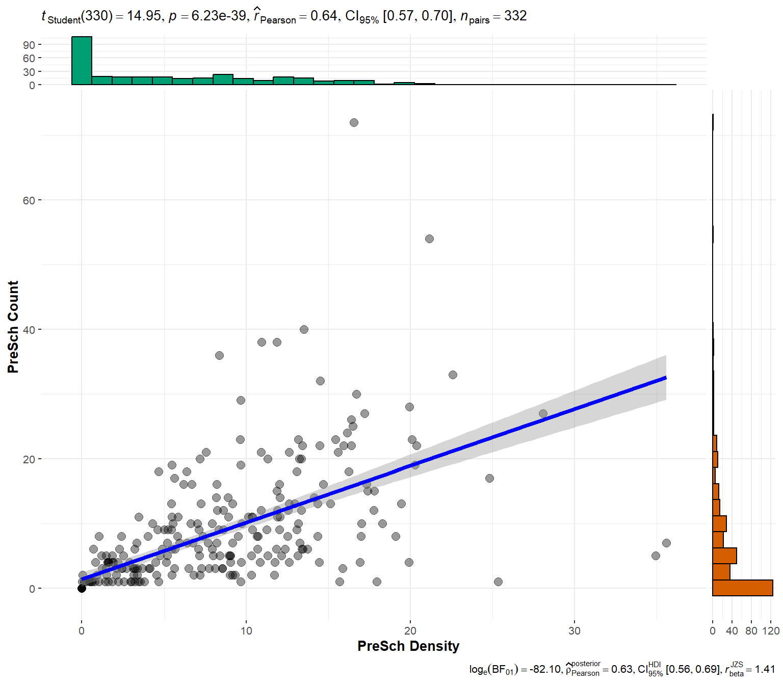
Using appropriate Exploratory Data Analysis (EDA) and Confirmatory Data Analysis (CDA) methods to explore and confirm the statistical relationship between Pre-school Density and Pre-school count.

Tip: Refer to ggscatterstats() of ggstatsplot package.

mpsz$`PreSch Density` <- as.numeric(as.character(mpsz19_shp$`PreSch Density`))
mpsz$`PreSch Count` <- as.numeric(as.character(mpsz19_shp$`PreSch Count`)) 
mpsz19_shp <- as.data.frame(mpsz19_shp)

ggscatterstats(data = mpsz19_shp,
               x = `PreSch Density`,
               y = `PreSch Count`,
               type = "parametric")

Working with Population Data

• The task
• The code

1. Visit and extract the latest Singapore Residents by Planning Area / Subzone, Age Group, Sex and Type of Dwelling from Singstat homepage.

popdata <- read_csv("data/respopagesextod2023.csv")

Data Wrangling

• The task
• The code

1. Write a code chunk to prepare a data.frame showing population by Planning Area and Planning subzone

popdata2023 <- popdata %>% 
  group_by(PA, SZ, AG) %>% 
  summarise(`POP`=sum(`Pop`)) %>%  
  ungroup() %>% 
  pivot_wider(names_from=AG,
              values_from = POP)

colnames(popdata2023)

 [1] "PA"          "SZ"          "0_to_4"      "10_to_14"    "15_to_19"   
 [6] "20_to_24"    "25_to_29"    "30_to_34"    "35_to_39"    "40_to_44"   
[11] "45_to_49"    "50_to_54"    "55_to_59"    "5_to_9"      "60_to_64"   
[16] "65_to_69"    "70_to_74"    "75_to_79"    "80_to_84"    "85_to_89"   
[21] "90_and_Over"

Data Processing

• The task
• The code

Write a code chunk to derive a tibble data.framewith the following fields PA, SZ, YOUNG, ECONOMY ACTIVE, AGED, TOTAL, DEPENDENCY where by:

• YOUNG: age group 0 to 4 until age groyup 20 to 24,
• ECONOMY ACTIVE: age group 25-29 until age group 60-64,
• AGED: age group 65 and above,
• TOTAL: all age group, and
• DEPENDENCY: the ratio between young and aged against economy active group.

popdata2023 <- popdata2023 %>%
  mutate(YOUNG=rowSums(.[3:6]) # Aged 0 - 24, 10 - 24
         +rowSums(.[14])) %>% # Aged 5 - 9
  mutate(`ECONOMY ACTIVE` = rowSums(.[7:13])+ # Aged 25 - 59
  rowSums(.[15])) %>%  # Aged 60 -64
  mutate(`AGED`=rowSums(.[16:21])) %>%
  mutate(`TOTAL`=rowSums(.[3:21])) %>%
  mutate(`DEPENDENCY`=(`YOUNG` + `AGED`)
  / `ECONOMY ACTIVE`) %>% 
  select(`PA`, `SZ`, `YOUNG`, 
         `ECONOMY ACTIVE`, `AGED`,
         `TOTAL`, `DEPENDENCY`)

Joining popdata2023 and mpsz19_shp

The code chunk below is used to change data in the PA and SZ fields into uppercase.

popdata2023 <- popdata2023 %>%
  mutate_at(.vars = vars(PA, SZ), 
          .funs = list(toupper)) 

The code chunk below is used to perform left-join whereby the join fields are SUBZONE_N from the mpsz19_shp sf data.frame and SZ from the popdata2023 data.frame.

mpsz_pop2023 <- left_join(mpsz19_shp, popdata2023,
                          by = c("SUBZONE_N" = "SZ"))

Choropleth Map of Dependency Ratio by Planning Subzone

• The map
• The code

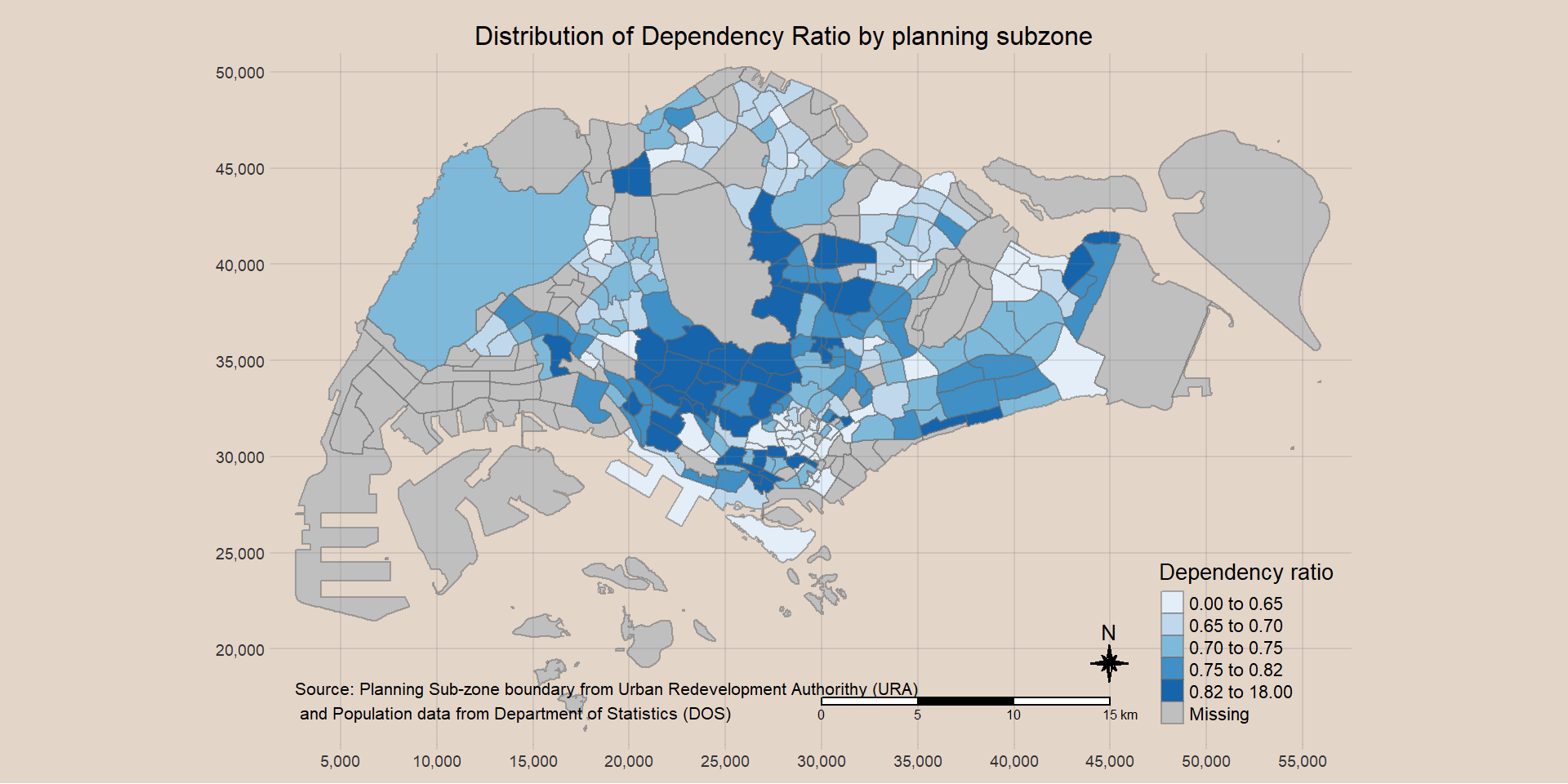
tm_shape(mpsz_pop2023)+
  
  tm_fill("DEPENDENCY", 
          style = "quantile", 
          palette = "Blues",
          title = "Dependency ratio") +
  
  tm_layout(main.title = "Distribution of Dependency Ratio by planning subzone",
            main.title.position = "center",
            main.title.size = 1,
            legend.title.size = 1,
            legend.height = 0.45, 
            legend.width = 0.35,
            bg.color = "#E4D5C9",
            frame = F) +
  
  tm_borders(alpha = 0.5) +
  tm_compass(type="8star", size = 1.5) +
  tm_scale_bar() +
  tm_grid(alpha =0.2) +
  tm_credits("Source: Planning Sub-zone boundary from Urban Redevelopment Authorithy (URA)\n and Population data from Department of Statistics (DOS)", 
             position = c("left", "bottom"))