In-class Exercise 5: Geographically Weighted Statistics - gwModel methods

Dr. Kam Tin Seong
Assoc. Professor of Information Systems(Practice)

School of Computing and Information Systems,
Singapore Management University

17 Sep 2024

Loading the package

In this in-class exercise, sf, spdep, tmap, tidyverse, knitr and GWmodel will be used.

• DIY
• The code

Using the step you leanred from previous hands-in, install and load the necessary R packages in R environment.

pacman::p_load(sf, spdep, tmap, tidyverse, knitr, GWmodel)

Preparing the Data

For this in-class exercise, Hunan shapefile and Hunan_2012 data file will be used.

• DIY
• Importing Hunan shapefile
• Importing Hunan_2012 table
• Joining Hunan and Hunan_2012

Using the steps you learned from previous hands-on, complete the following tasks:

• import Hunan shapefile and parse it into a sf polygon feature object.
• import Hunan_2012.csv file parse it into a tibble data.frame.
• join Hunan and Hunan_2012 data.frames.

hunan_sf <- st_read(dsn = "data/geospatial", 
                 layer = "Hunan")

Reading layer `Hunan' from data source 
  `D:\tskam\is415-gaa\In-class_Ex\In-class_Ex05\data\geospatial' 
  using driver `ESRI Shapefile'
Simple feature collection with 88 features and 7 fields
Geometry type: POLYGON
Dimension:     XY
Bounding box:  xmin: 108.7831 ymin: 24.6342 xmax: 114.2544 ymax: 30.12812
Geodetic CRS:  WGS 84

hunan2012 <- read_csv("data/aspatial/Hunan_2012.csv")

hunan_sf <- left_join(hunan_sf, hunan2012) %>%
  select(1:3, 7, 15, 16, 31, 32)

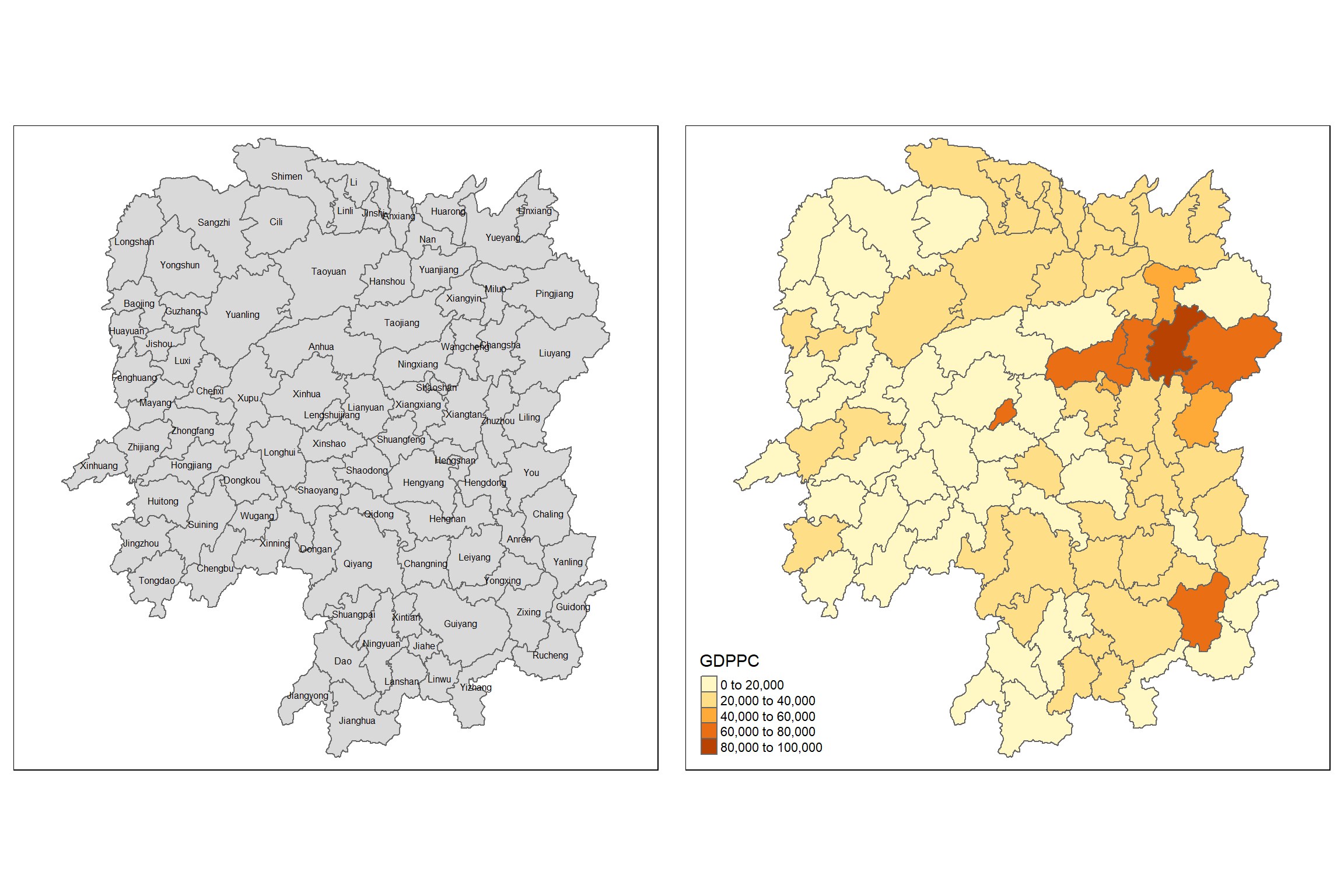
Mapping GDPPC

• DIY
• The code

Using the steps you learned from Hands-on Exercise 5, prepare a choropleth map showing the geographic distribution of GDPPC of Hunan Province.

basemap <- tm_shape(hunan_sf) +
  tm_polygons() +
  tm_text("NAME_3", size=0.5)

gdppc <- qtm(hunan, "GDPPC")
tmap_arrange(basemap, gdppc, asp=1, ncol=2)

Converting to SpatialPolygonDataFrame

Note

GWmodel presently is built around the older sp and not sf formats for handling spatial data in R.

hunan_sp <- hunan_sf %>%
  as_Spatial()

Geographically Weighted Summary Statistics with adaptive bandwidth

Determine adaptive bandwidth

• Cross-validation
• AIC

bw_CV <- bw.gwr(GDPPC ~ 1, 
             data = hunan_sp,
             approach = "CV",
             adaptive = TRUE, 
             kernel = "bisquare", 
             longlat = T)

Adaptive bandwidth: 62 CV score: 15515442343 
Adaptive bandwidth: 46 CV score: 14937956887 
Adaptive bandwidth: 36 CV score: 14408561608 
Adaptive bandwidth: 29 CV score: 14198527496 
Adaptive bandwidth: 26 CV score: 13898800611 
Adaptive bandwidth: 22 CV score: 13662299974 
Adaptive bandwidth: 22 CV score: 13662299974 

bw_CV

[1] 22

bw_AIC <- bw.gwr(GDPPC ~ 1, 
             data = hunan_sp,
             approach ="AIC",
             adaptive = TRUE, 
             kernel = "bisquare", 
             longlat = T)

Adaptive bandwidth (number of nearest neighbours): 62 AICc value: 1923.156 
Adaptive bandwidth (number of nearest neighbours): 46 AICc value: 1920.469 
Adaptive bandwidth (number of nearest neighbours): 36 AICc value: 1917.324 
Adaptive bandwidth (number of nearest neighbours): 29 AICc value: 1916.661 
Adaptive bandwidth (number of nearest neighbours): 26 AICc value: 1914.897 
Adaptive bandwidth (number of nearest neighbours): 22 AICc value: 1914.045 
Adaptive bandwidth (number of nearest neighbours): 22 AICc value: 1914.045 

bw_AIC

[1] 22

Geographically Weighted Summary Statistics with adaptive bandwidth

Computing geographically wieghted summary statistics

gwstat <- gwss(data = hunan_sp,
               vars = "GDPPC",
               bw = bw_AIC,
               kernel = "bisquare",
               adaptive = TRUE,
               longlat = T)

Geographically Weighted Summary Statistics with adaptive bandwidth

Preparing the output data

Code chunk below is used to extract SDF data table from gwss object output from gwss(). It will be converted into data.frame by using as.data.frame().

gwstat_df <- as.data.frame(gwstat$SDF)

Next, cbind() is used to append the newly derived data.frame onto hunan_sf sf data.frame.

hunan_gstat <- cbind(hunan_sf, gwstat_df)

Geographically Weighted Summary Statistics with adaptive bandwidth

Visualising geographically weighted summary statistics

• The Geographically Weighted Mean
• The code

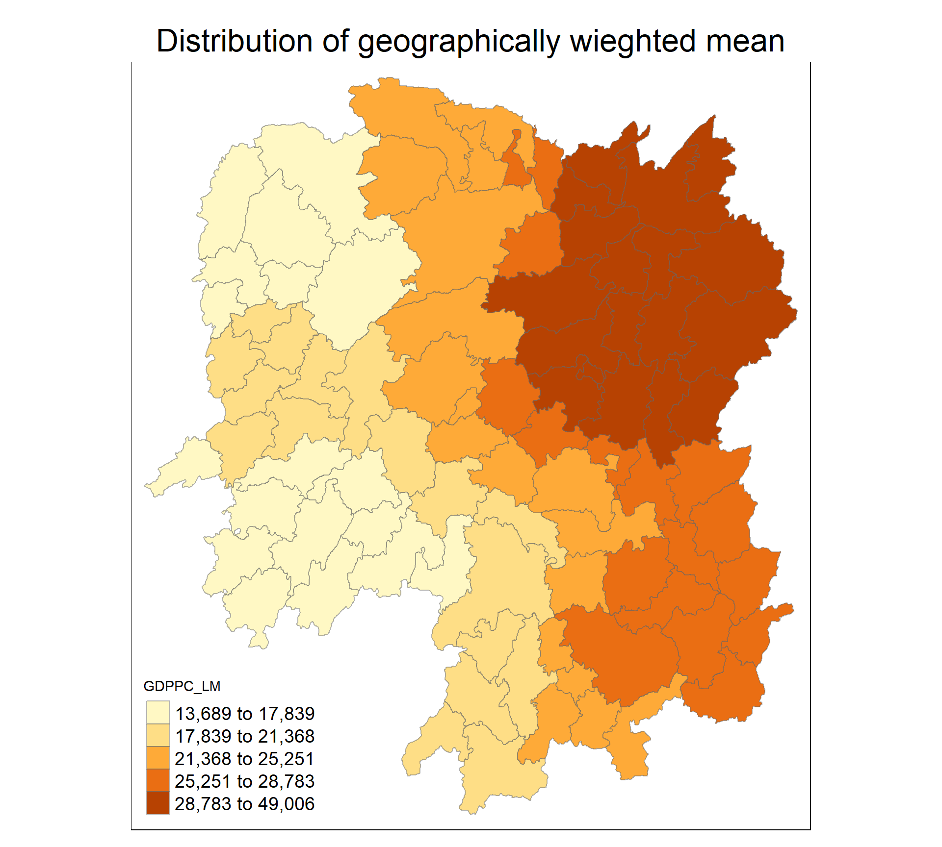
tm_shape(hunan_gstat) +
  tm_fill("GDPPC_LM",
          n = 5,
          style = "quantile") +
  tm_borders(alpha = 0.5) +
  tm_layout(main.title = "Distribution of geographically wieghted mean",
            main.title.position = "center",
            main.title.size = 2.0,
            legend.text.size = 1.2,
            legend.height = 1.50, 
            legend.width = 1.50,
            frame = TRUE)

Geographically Weighted Summary Statistics with fixed

Determine fixed bandwidth

• Cross-validation
• AIC

bw_CV <- bw.gwr(GDPPC ~ 1, 
             data = hunan_sp,
             approach = "CV",
             adaptive = FALSE, 
             kernel = "bisquare", 
             longlat = T)

Fixed bandwidth: 357.4897 CV score: 16265191728 
Fixed bandwidth: 220.985 CV score: 14954930931 
Fixed bandwidth: 136.6204 CV score: 14134185837 
Fixed bandwidth: 84.48025 CV score: 13693362460 
Fixed bandwidth: 52.25585 CV score: Inf 
Fixed bandwidth: 104.396 CV score: 13891052305 
Fixed bandwidth: 72.17162 CV score: 13577893677 
Fixed bandwidth: 64.56447 CV score: 14681160609 
Fixed bandwidth: 76.8731 CV score: 13444716890 
Fixed bandwidth: 79.77877 CV score: 13503296834 
Fixed bandwidth: 75.07729 CV score: 13452450771 
Fixed bandwidth: 77.98296 CV score: 13457916138 
Fixed bandwidth: 76.18716 CV score: 13442911302 
Fixed bandwidth: 75.76323 CV score: 13444600639 
Fixed bandwidth: 76.44916 CV score: 13442994078 
Fixed bandwidth: 76.02523 CV score: 13443285248 
Fixed bandwidth: 76.28724 CV score: 13442844774 
Fixed bandwidth: 76.34909 CV score: 13442864995 
Fixed bandwidth: 76.24901 CV score: 13442855596 
Fixed bandwidth: 76.31086 CV score: 13442847019 
Fixed bandwidth: 76.27264 CV score: 13442846793 
Fixed bandwidth: 76.29626 CV score: 13442844829 
Fixed bandwidth: 76.28166 CV score: 13442845238 
Fixed bandwidth: 76.29068 CV score: 13442844678 
Fixed bandwidth: 76.29281 CV score: 13442844691 
Fixed bandwidth: 76.28937 CV score: 13442844698 
Fixed bandwidth: 76.2915 CV score: 13442844676 
Fixed bandwidth: 76.292 CV score: 13442844679 
Fixed bandwidth: 76.29119 CV score: 13442844676 
Fixed bandwidth: 76.29099 CV score: 13442844676 
Fixed bandwidth: 76.29131 CV score: 13442844676 
Fixed bandwidth: 76.29138 CV score: 13442844676 
Fixed bandwidth: 76.29126 CV score: 13442844676 
Fixed bandwidth: 76.29123 CV score: 13442844676 

bw_CV

[1] 76.29126

bw_AIC <- bw.gwr(GDPPC ~ 1, 
             data = hunan_sp,
             approach ="AIC",
             adaptive = FALSE, 
             kernel = "bisquare", 
             longlat = T)

Fixed bandwidth: 357.4897 AICc value: 1927.631 
Fixed bandwidth: 220.985 AICc value: 1921.547 
Fixed bandwidth: 136.6204 AICc value: 1919.993 
Fixed bandwidth: 84.48025 AICc value: 1940.603 
Fixed bandwidth: 168.8448 AICc value: 1919.457 
Fixed bandwidth: 188.7606 AICc value: 1920.007 
Fixed bandwidth: 156.5362 AICc value: 1919.41 
Fixed bandwidth: 148.929 AICc value: 1919.527 
Fixed bandwidth: 161.2377 AICc value: 1919.392 
Fixed bandwidth: 164.1433 AICc value: 1919.403 
Fixed bandwidth: 159.4419 AICc value: 1919.393 
Fixed bandwidth: 162.3475 AICc value: 1919.394 
Fixed bandwidth: 160.5517 AICc value: 1919.391 

bw_AIC

[1] 160.5517

Geographically Weighted Summary Statistics with fixed

Computing adaptive bandwidth

gwstat <- gwss(data = hunan_sp,
               vars = "GDPPC",
               bw = bw_AIC,
               kernel = "bisquare",
               adaptive = FALSE,
               longlat = T)

Geographically Weighted Summary Statistics with fixed bandwidth

Preparing the output data

Code chunk below is used to extract SDF data table from gwss object output from gwss(). It will be converted into data.frame by using as.data.frame().

gwstat_df <- as.data.frame(gwstat$SDF)

Next, cbind() is used to append the newly derived data.frame onto hunan_sf sf data.frame.

hunan_gstat <- cbind(hunan_sf, gwstat_df)

Geographically Weighted Summary Statistics with fixed

Visualising geographically weighted summary statistics

• The Geographically Weighted Mean
• The code

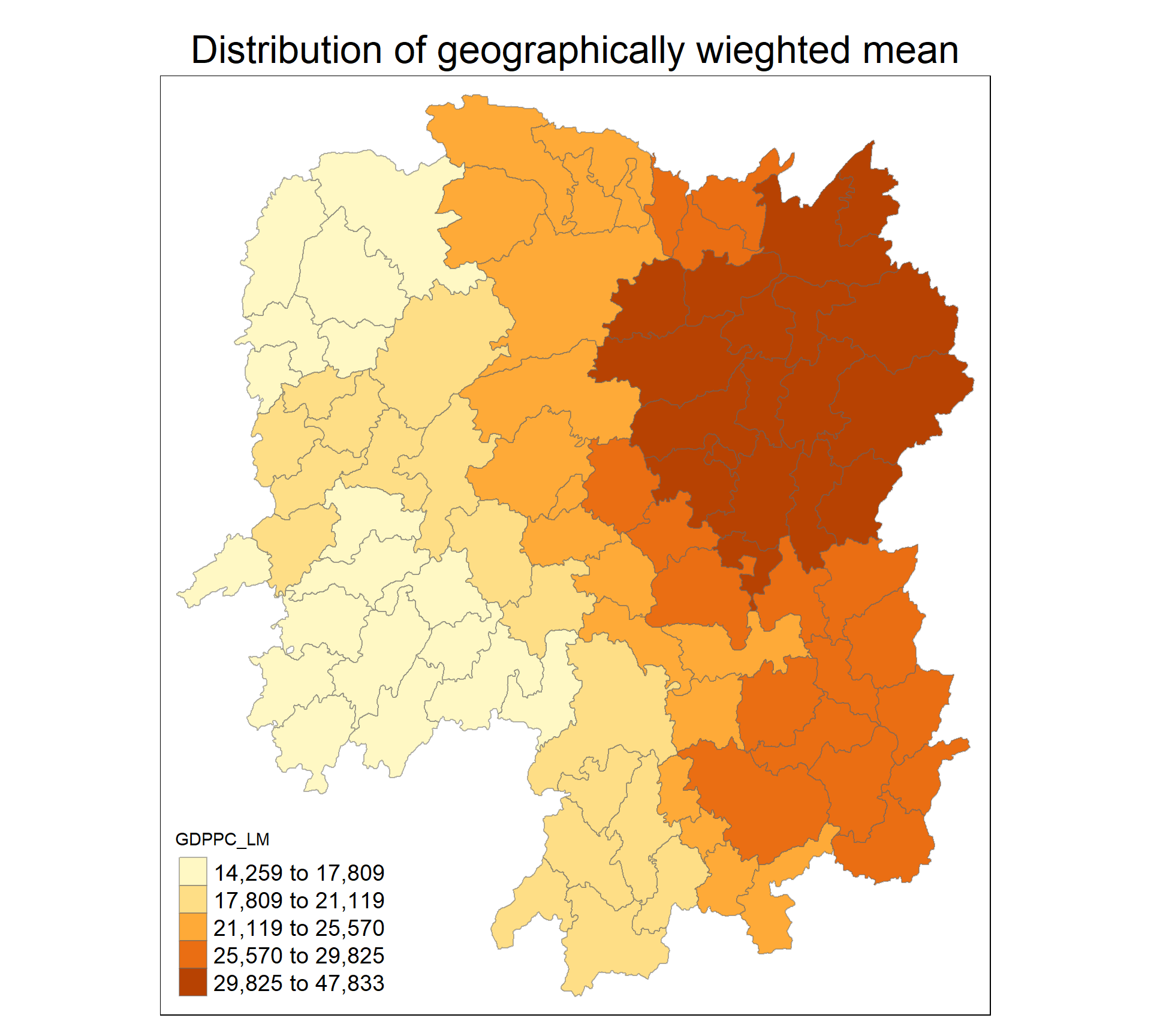
tm_shape(hunan_gstat) +
  tm_fill("GDPPC_LM",
          n = 5,
          style = "quantile") +
  tm_borders(alpha = 0.5) +
  tm_layout(main.title = "Distribution of geographically wieghted mean",
            main.title.position = "center",
            main.title.size = 2.0,
            legend.text.size = 1.2,
            legend.height = 1.50, 
            legend.width = 1.50,
            frame = TRUE)